-
 Benyahia Mohammed Oussama authoredBenyahia Mohammed Oussama authored
- TD 2: GAN & Diffusion
- MSO 3.4 Machine Learning
- Overview
- Part 1: DC-GAN
- Implemented Modifications
- Examples of Generated Images:
- Question: How to Control the Generated Digit?
- Generator Modifications
- Discriminator Modifications
- Training Process Update
- Implementing a cGAN with a Multi-Class Discriminator
- Algorithm Comparison
- Examples of Digit (3) Generated by cGAN with Real/Fake Discriminator:
- Examples of Digit (3) Generated by cGAN with Multi-Class Discriminator:
- Conclusion
- References
- Part 2: Conditional GAN (cGAN) with U-Net
- Generator
- U-Net Overview:
- Architecture & Implementation:
- Question:
- Question:
- Explanation:
- Discriminator
- PatchGAN Overview:
- Question:
- Results Comparison: 100 vs. 200 Epochs
- 1. Training Performance
- 2. Evaluation Performance
- Conclusion & Observations
- Example image of training set at 100 and 200 epochs:
- Example images of evaluation set at 100 and 200 epochs:
- Part 3: Diffusion Models
- Overview of Diffusion Models
- The Diffusion Process
- Noise Scheduler
- Architecture for Diffusion Model: UNet2DModel (Diffusion Model)
- Training the Model
- UNet Model Architecture
- Comparison: UNet Model vs. Diffusion UNet (DDPM)
- Results
- Analysis: Noise Prediction and Image Denoising Performance
- Conclusion
- Part 4: What About Those Beautiful Images?
- Strong Model: Stable Diffusion 3.5 with Quantization
- Smaller Model: OFA-Sys Small-Stable-Diffusion
- Conclusion
- How to submit your Work ?
TD 2: GAN & Diffusion
MSO 3.4 Machine Learning
Overview
This project explores generative models for images, focusing on Generative Adversarial Networks (GANs) and Diffusion models. The objective is to understand their implementation, analyze specific architectures, and apply different training strategies for generating and denoising images, both with and without conditioning.
Part 1: DC-GAN
In this section, we study the fundamentals of Generative Adversarial Networks through a Deep Convolutional GAN (DCGAN). We follow the tutorial: DCGAN Tutorial.
We generate handwritten digits using the MNIST dataset available in the torchvision package: MNIST Dataset.
Implemented Modifications
- Adapted the tutorial's code to work with the MNIST dataset.
- Displayed loss curves for both the generator and the discriminator over training steps.
- Compared generated images with real MNIST dataset images.
Examples of Generated Images:

Question: How to Control the Generated Digit?
To control which digit the generator produces, we implement a Conditional GAN (cGAN) with the following modifications:
Generator Modifications
- Instead of using only random noise, we concatenate a class label (one-hot encoded or embedded) with the noise vector.
- This allows the generator to learn to produce specific digits based on the provided label.
Discriminator Modifications
- Instead of just distinguishing real from fake, the discriminator is modified to classify images as digits (0-9) or as generated (fake).
- It outputs a probability distribution over 11 classes (10 digits + 1 for generated images).
Training Process Update
- The generator is trained to fool the discriminator while generating images that match the correct class label.
- A categorical cross-entropy loss is used for the discriminator instead of a binary loss since it performs multi-class classification.
- The loss function encourages the generator to produce well-classified digits.
Implementing a cGAN with a Multi-Class Discriminator
To enhance image generation and reduce ambiguities between similar digits (e.g., 3 vs 7), we introduce a multi-class discriminator that classifies generated images into one of the 10 digit categories or as fake.
Algorithm Comparison
| Model | Description | Result |
|---|---|---|
| cGAN | The generator learns to produce images conditioned on the class label. The discriminator only distinguishes real from fake. | Can generate realistic digits but sometimes ambiguous (e.g., confusion between 3 and 7). |
| cGAN with Multi-Class Discriminator | The generator produces class-conditioned digits, and the discriminator learns to classify images into one of 10 digit categories or as fake. | Improves image quality and reduces digit ambiguity. |
Examples of Digit (3) Generated by cGAN with Real/Fake Discriminator:

Examples of Digit (3) Generated by cGAN with Multi-Class Discriminator:

Conclusion
- GANs enable the generation of realistic handwritten digits.
- Adding conditioning via a cGAN allows control over the generated digit.
- Using a multi-class discriminator improves digit differentiation and reduces ambiguities.
References
Here is the corrected version with only the necessary adjustments:
Part 2: Conditional GAN (cGAN) with U-Net
Generator
In the cGAN architecture, the generator chosen is a U-Net.
U-Net Overview:
- A U-Net takes an image as input and outputs another image.
- It consists of two main parts: an encoder and a decoder.
- The encoder reduces the image dimension to extract main features.
- The decoder reconstructs the image using these features.
- Unlike a simple encoder-decoder model, U-Net has skip connections that link encoder layers to corresponding decoder layers. These allow the decoder to use both high-frequency and low-frequency information.
Architecture & Implementation:
The encoder takes a colored picture (3 channels: RGB), processes it through a series of convolutional layers, and encodes the features. The decoder then reconstructs the image using transposed convolutional layers, utilizing skip connections to enhance details.

Question:
Knowing that the input and output images have a shape of 256x256 with 3 channels, what will be the dimension of the feature map "x8"?
Answer: The dimension of the feature map x8 is [numBatch, 512, 32, 32].
Question:
Why are skip connections important in the U-Net architecture?
Explanation:
Skip connections link encoder and decoder layers, improving the model in several ways:
- Preserving Spatial Resolution: Helps retain fine details that may be lost during encoding.
- Preventing Information Loss: Transfers important features from the encoder to the decoder.
- Improving Performance: Combines high-level and low-level features for better reconstruction.
- Mitigating Vanishing Gradient: Eases training by allowing gradient flow through deeper layers.
Discriminator
In the cGAN architecture, we use a PatchGAN discriminator instead of a traditional binary classifier.
PatchGAN Overview:
- Instead of classifying the entire image as real or fake, PatchGAN classifies N × N patches of the image.
- The size N depends on the number of convolutional layers in the network:
| Layers | Patch Size |
|---|---|
| 1 | 16×16 |
| 2 | 34×34 |
| 3 | 70×70 |
| 4 | 142×142 |
| 5 | 286×286 |
| 6 | 574×574 |
For this project, we use a 70×70 PatchGAN.

Question:
How many learnable parameters does this neural network have?
-
conv1:
- Input channels: 6
- Output channels: 64
- Kernel size: 4×4
- Parameters in conv1 : (4×4×6+1(bias))×64 = 6208
-
conv2:
- Weights: 4 × 4 × 64 × 128 = 131072
- Biases: 128
- BatchNorm: (scale + shift) for 128 channels: 2 × 128 = 256
- Parameters in conv2: 131072 + 128 + 256 = 131456
-
conv3:
- Weights: 4 × 4 × 128 × 256 = 524288
- Biases: 256
- BatchNorm: (scale + shift) for 256 channels: 2 × 256 = 512
- Parameters in conv3: 524288 + 256 + 512 = 525056
-
conv4:
- Weights: 4 × 4 × 256 × 512 = 2097152
- Biases: 512
- BatchNorm: (scale + shift) for 512 channels: 2 × 512 = 1024
- Parameters in conv4: 2097152 + 512 + 1024 = 2098688
-
out:
- Weights: 4 × 4 × 512 × 1 = 8192
- Biases: 1
- Parameters in out: 8192 + 1 = 8193
Total Learnable Parameters:
6208 + 131456 + 525056 + 2098688 + 8193 = 2,769,601
Results Comparison: 100 vs. 200 Epochs
1. Training Performance
-
100 Epochs:
- The generator produces images that resemble the target facades.
- Some fine details may be missing, and slight noise is present.
-
200 Epochs:
- The generated facades have more details and refined structures.
- Improved high-frequency details make outputs closer to target images.
- Less noise, but minor artifacts may still exist.
2. Evaluation Performance
-
100 Epochs:
- Struggles with realistic facades on unseen masks.
- Noticeable noise, but sometimes less than the 200-epoch model.
- Some structures exist but lack consistency.
-
200 Epochs:
- Overfits to training data, leading to poor generalization.
- Instead of realistic facades, it reuses training patches, causing noisy outputs.
Conclusion & Observations
- Improved Detail at 200 Epochs: Better training mask generation.
- Overfitting Issue: Generalization is poor beyond 100 epochs.
- Limited Dataset Size (378 Images): Restricts model’s diversity and quality.
Example image of training set at 100 and 200 epochs:

Example images of evaluation set at 100 and 200 epochs:

Part 3: Diffusion Models
Diffusion models represent a cutting-edge approach in generative modeling, focusing on the transformation of random noise into realistic data through an iterative denoising process. The reverse diffusion process begins with a noisy image and gradually refines it into a high-quality image using a trained neural network. These models have gained significant attention due to their ability to outperform GANs in generating diverse and high-fidelity images.
Overview of Diffusion Models
This project explores Denoising Diffusion Probabilistic Models (DDPMs), which are widely used for image noise prediction. The fundamental idea is to progressively apply noise over multiple timesteps and then train a neural network to reverse this process. The model learns to predict and remove noise at each timestep, effectively reconstructing a clean image.
The Diffusion Process
- Forward Diffusion Process: Noise is incrementally added to an image over a series of timesteps. As the number of steps increases, the image becomes progressively noisier until it reaches a state of pure noise.
- Reverse Diffusion Process: A neural network is trained to undo the noise addition process by predicting and removing noise step by step, ultimately recovering the original image.
Noise Scheduler
To regulate the diffusion process, we use a noise scheduler, which defines the amount of noise added at each timestep. The model is trained on the MNIST dataset, as introduced in Part 1 of this project.
Architecture for Diffusion Model: UNet2DModel (Diffusion Model)
The UNet2DModel is specifically designed for diffusion-based denoising tasks. Key architectural features include:
-
Time Conditioning: The
time_projandtime_embeddingmodules encode timestep information, crucial for learning the progressive denoising process. -
ResNet Blocks: Instead of simple convolution layers, each downsampling and upsampling step integrates
ResNetBlock2Dwith GroupNorm and SiLU (Swish) activation, enhancing robustness. - SiLU Activation: Chosen over LeakyReLU or ReLU for smoother gradients.
- GroupNorm: Provides more stable training compared to BatchNorm in diffusion models.
Training the Model
We train the diffusion model using the diffusers library on the MNIST dataset. Performance is assessed across different epochs to analyze the quality of generated images.
Bonus: We also evaluate a standard UNet Model by inputting the timestep embedding along with the noisy image. This UNet follows an encoder-decoder structure and is typically used for image-to-image translation.
UNet Model Architecture
The UNet Model, in contrast to the diffusion model, aims to predict and remove noise in a single step. Key features include:
- Encoder-Decoder Structure: Employs Conv2D + BatchNorm + LeakyReLU for downsampling and ConvTranspose2D + BatchNorm + ReLU for upsampling.
- Skip Connections: Each downsampling layer has a corresponding upsampling layer that concatenates feature maps.
- Dropout Layers: Enhance regularization to prevent overfitting.
- LeakyReLU Activation: Improves feature extraction in the downsampling process.
Comparison: UNet Model vs. Diffusion UNet (DDPM)
| Feature | UNet Model | Diffusion UNet (DDPM) |
|---|---|---|
| Primary Task | Image-to-image translation | Image denoising via diffusion |
| Downsampling | Strided Conv2D + BatchNorm + LeakyReLU | ResNet Blocks + GroupNorm + SiLU |
| Upsampling | Transpose Conv2D | Interpolation + Conv2D |
| Activation Function | LeakyReLU (down), ReLU (up), Tanh (output) | SiLU (Swish) |
| Normalization | BatchNorm | GroupNorm |
| Skip Connections | Yes | Yes |
| Time Embedding | No | Yes |
Results
Diffusion UNet2D Model

UNet Model

Analysis: Noise Prediction and Image Denoising Performance
Both models leverage the UNet architecture but employ different strategies for noise removal:
- Diffusion UNet2D Model: Works iteratively, progressively removing noise in multiple steps. This allows it to generate high-quality images but at the cost of increased computational complexity.
- UNet Model: Predicts and removes noise in a single step, making it significantly faster. However, it struggles to accurately predict the noise pattern, leading to incomplete denoising and residual artifacts in the final output.
Conclusion
The UNet2DModel (Diffusion Model) provides superior denoising quality due to its iterative refinement process, making it ideal for high-quality image generation. However, its computational cost is high, limiting its applicability in real-time scenarios. On the other hand, the UNet Model is computationally efficient, offering faster inference, but its denoising performance is subpar, resulting in images where numbers become unrecognizable due to residual noise.
Part 4: What About Those Beautiful Images?
In this experiment, we compared the performance of two models: a large pre-trained model (Stable Diffusion 3.5 with quantization) and a smaller model (OFA-Sys small-stable-diffusion).
Strong Model: Stable Diffusion 3.5 with Quantization
Using 4-bit quantization, this model produced high-quality and creative images from simple textual prompts, even with reduced memory requirements. We tested the model with prompts like:
- "Underwater wheeled bee"
- "Monster buys lollipop"
- "Imagine a world without eggs"
The results were visually appealing and imaginative, showcasing the model's capability to generate intricate and high-quality images.
Example Results from Stable Diffusion 3.5:
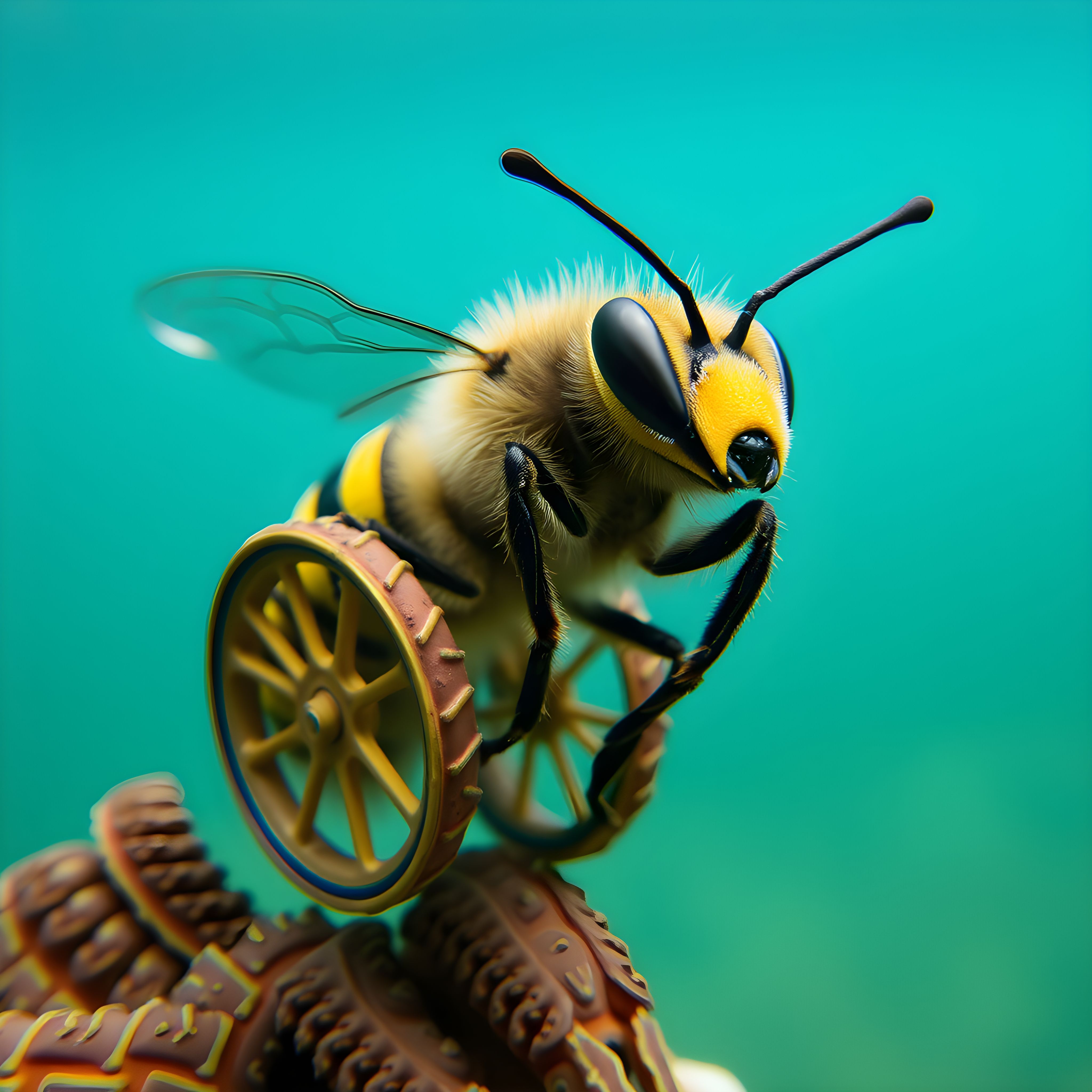
Underwater wheeled bee from large model
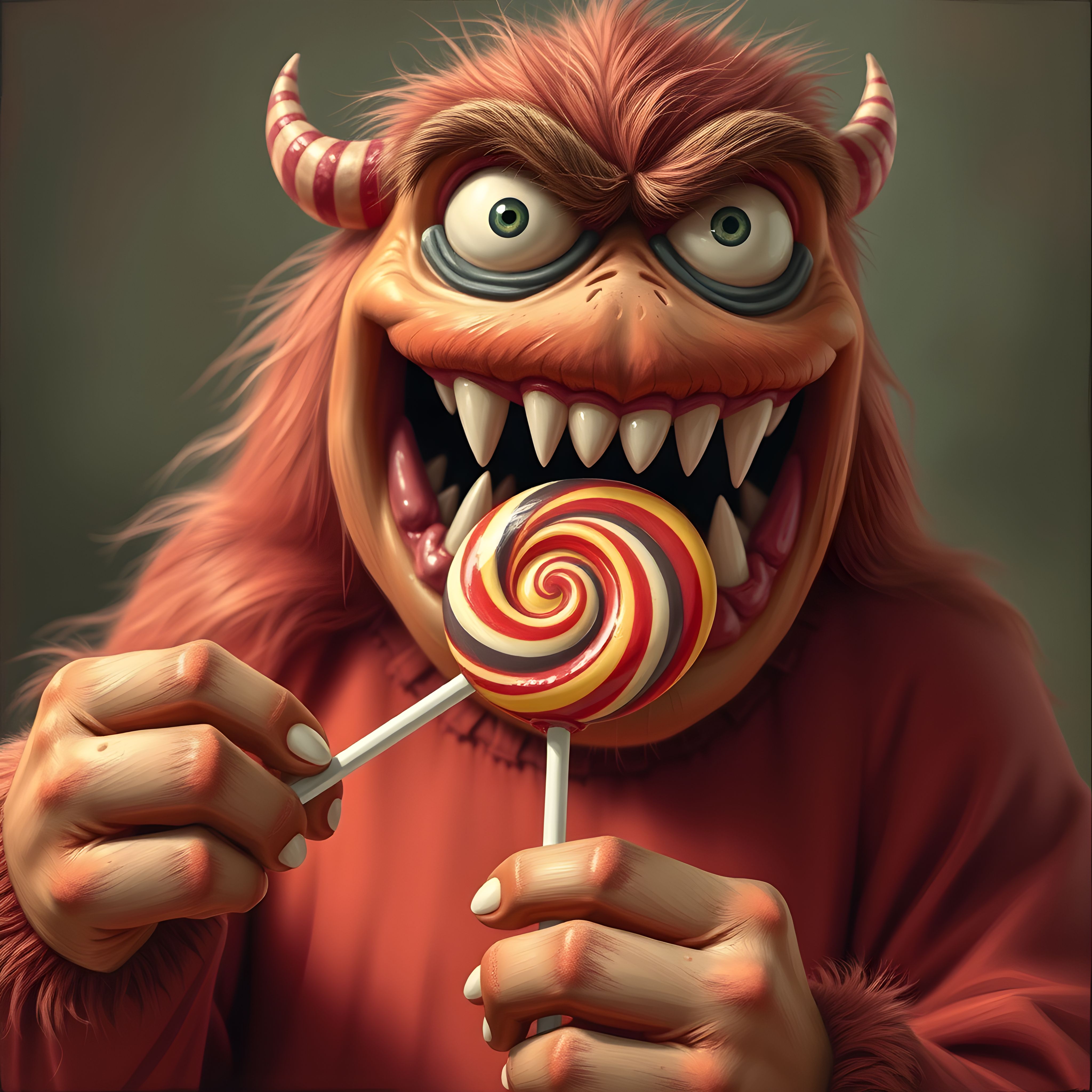
Monster buys lollipop from large model
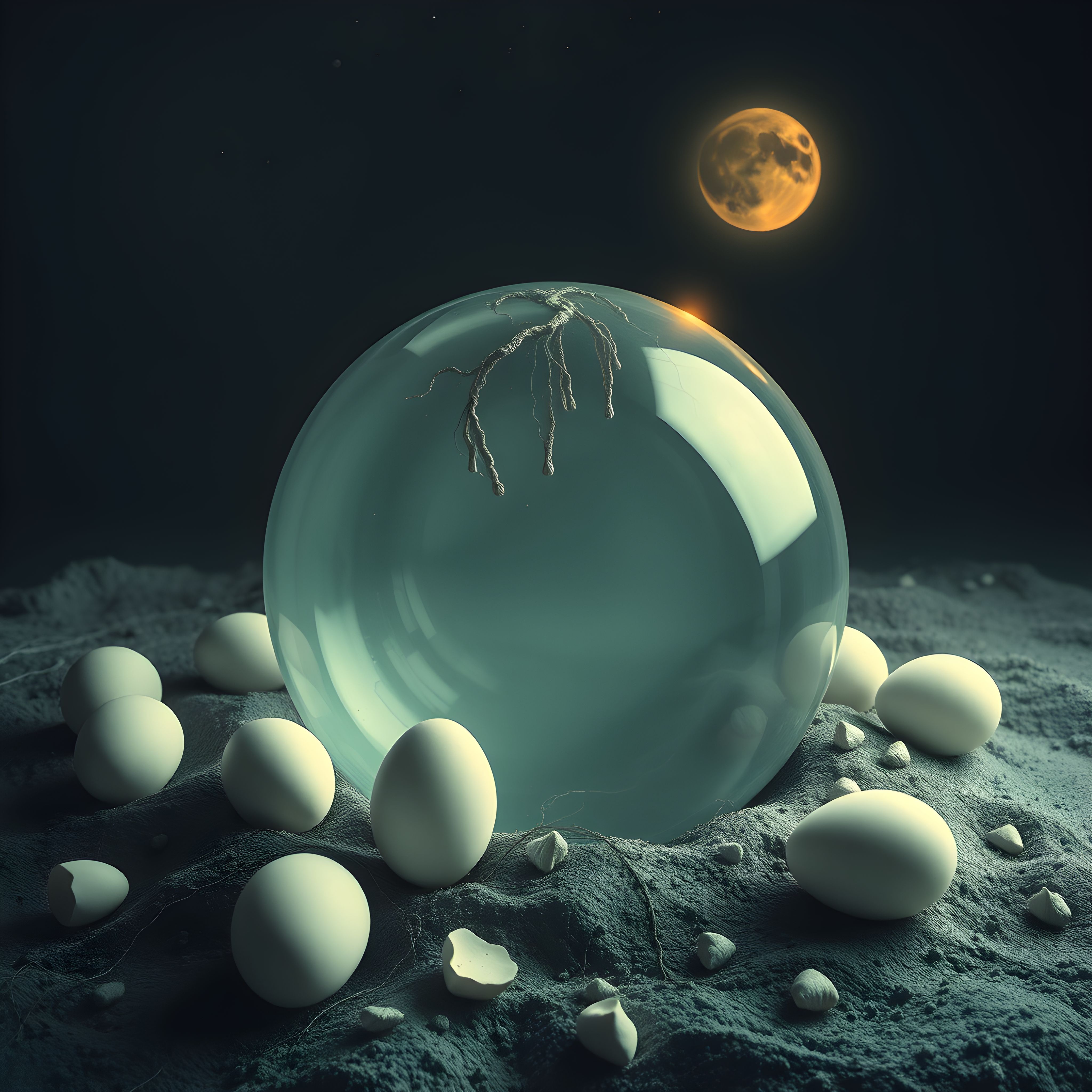
Imagine a world without eggs from large model
Smaller Model: OFA-Sys Small-Stable-Diffusion
While the smaller model generated images, the quality and creativity were noticeably lower. The images lacked the detail and originality seen with the larger model, confirming that smaller models are less capable of handling complex, creative prompts.
Example Results from OFA-Sys Small-Stable-Diffusion:

Underwater wheeled bee from smaller model

Monster buys lollipop from smaller model

Imagine a world without eggs from smaller model
Conclusion
The experiment demonstrates that larger models, like Stable Diffusion 3.5, produce superior image quality and creativity. However, smaller models can still be useful in scenarios with hardware limitations, though they fall short in terms of detail and imagination when compared to their larger counterparts.
How to submit your Work ?
This work must be done individually. The expected output is a private repository named gan-diffusion on https://gitlab.ec-lyon.fr. It must contain your notebook (or python files) and a README.md file that explains briefly the successive steps of the project. Don't forget to add your teacher as developer member of the project. The last commit is due before 11:59 pm on Wednesday, April 9th, 2025. Subsequent commits will not be considered.